
Geographical Information Systems such as QGIS are common in the typical archaeologist’s toolbox. However, the complexities of our datasets mean that we need additional tools to identify patterns in time and space.
Imagine that you are working with a set of points in a vector format such as a Shapefile. It can be a set of settlements, C14 dates or shipwrecks…it doesn’t matter; you will want to combine spatial analysis with other methods. This is particularly true when you are trying to get a feeling of the dataset by performing Exploratory Data Analysis, so you need to compile summary statistics and create some meaningful visualisations.
My personal approach is to combine QGIS with R and exploit the awesome ggplot package to get some insight into the dataset beyond spatial patterns. R has some nice spatial functionality, but the cool thing is to integrate these methods with other plots to get a general picture of the case study you are studying.
Example: Aircraft crashes in the Orkney islands
The Orkney islands were a key location for the British war effort during the Two World Wars because it hosted Scapa Flow: the main naval base of the Royal Navy. For this reason it saw an intense aerial activity of all sorts: squadrons defending the base, German bombers attacking it, aircraft carrier operations…you name it. Inevitably this activity generated aircraft crashes due to accidents and combat and these events have been compiled by different initiatives such as the Project Adair-Whitaker or the ARGOS group.
I created a nice Shapefile of aircraft crash sites based on the information provided by Canmore. How can I explore the dataset beyond the spatial dynamics? How many German aircrafts were shot down? What types and squadrons sustained more losses? Let’s take a look!
Download Data
The first thing to do is to load the Shapefile. This format requires of several files so I created a zip file with all the set. First of all we need to download it to a temporary directory and extract its contents:
[generic linenumbers=”False”] tmp <- tempdir()url <- "https://github.com/xrubio/pastByNumbers/raw/master/data/aircraft_orkney.zip"
file <- basename(url)
download.file(url, file)
unzip(file, exdir = tmp)
[/generic]
Load the spatial data
We will use the rgdal library to load the contents of the Shapefile into R:
[generic linenumbers=”False”]
library(rgdal)
aircraftShp <- readOGR(dsn = tmp, layer="aircraft_orkney")
str(aircraftShp)
[/generic]
aircraftShp is a variable of type SpatialPointsDataFrame from package sp. It is a container of some interesting information such as the bounding box delimiting our spatial entities or the Coordinate Reference System that it is being used. Ideally we would like to get the attributes of the spatial entities as a data frame so we can use it with most R packages:
[generic linenumbers=”False”] aircraft <- as.data.frame(aircraftShp)str(aircraft)
[/generic]
Maps and planes
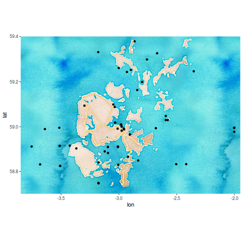
First of all let’s plot the spatial coordinates of the aircraft crash sites against a nice background. I created a rectangle location based on the bounding box of aircraftShp:
[generic linenumbers=”False”] aircraftShp@bboxlocation <- c(-3.85, 58.7, -1.95, 59.4)
[/generic]
We can use ggmap to download the background:
[generic linenumbers=”False”]
library(ggplot2)
library(ggmap)
bgMap <- get_map(location=location, source="stamen", maptype="watercolor")
ggmap(bgMap) + geom_point(data=aircraft, aes(x=coords.x1, y=coords.x2))
[/generic]
Exploring other dimensions
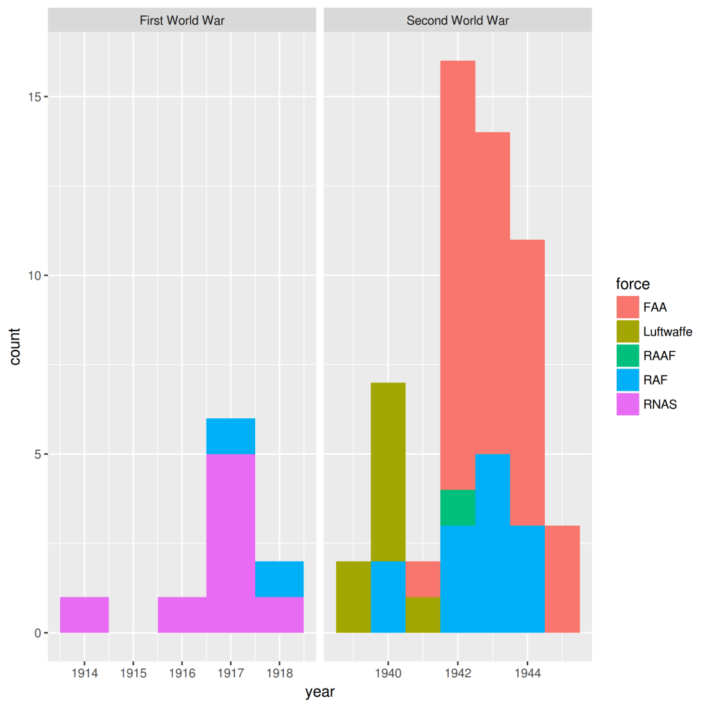
This is ok but it is something we can already do with any GIS so…what’s the deal? The thing is that aircraft is an R Data Frame so we can plot any variable using a graphic library, something that R does way better than any GIS. For example, let’s take a look at the temporal dimension:
[generic linenumbers=”False”] ggplot(aircraft, aes(x=year, fill=force)) + geom_histogram(binwidth=1) + facet_wrap(~war, scales=”free_x”)[/generic]
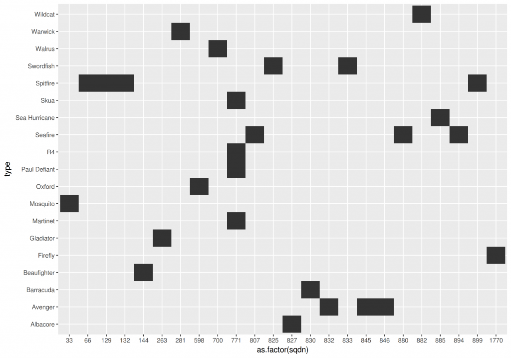
We can also create a table of planes used by the different British squadrons that suffered losses:
[generic linenumbers=”False”] ggplot(na.omit(aircraft), aes(y=type, col=force, x=as.factor(sqdn))) + geom_raster()[/generic]
Combining everything
We can finally create an infographic combining space, time and other stuff with the library gridExtra:
First, we create nice version of the plots we just saw:
[generic linenumbers=”False”] g1 <- ggmap(bgMap, extent="panel", darken = c(.4,"white")) + geom_point(data=aircraft, aes(x=coords.x1, y=coords.x2, col=war), size=2) + geom_text(data=aircraft, aes(x=coords.x1, y=coords.x2,label=type), family = "Trebuchet MS", color="grey40", check_overlap=T, nudge_y=0.01) + theme(legend.position="bottom") + ggtitle("aircraft losses") + xlab("") + ylab("") + scale_color_manual(values=c("indianred2", "goldenrod1"))g2 <- ggplot(na.omit(aircraft), aes(y=type, col=force, x=as.factor(sqdn))) + geom_point(size=3) + theme_bw() + theme(legend.position="bottom") + xlab("squadron") + ylab("") + ggtitle("Britain – aircraft types per squadron")
g3 <- ggplot(aircraft, aes(x=year, fill=force)) + geom_histogram(binwidth=1, col="black") + facet_wrap(~war, scales="free_x", ncol=1) + theme_bw() + theme(legend.position="bottom") + ggtitle("losses per year") + xlab("") + ylab("")
[/generic]
And we can then combine the 3 plots into a nice visualization:
[generic linenumbers=”False”]
library(gridExtra)
grid.arrange(arrangeGrob(arrangeGrob(g1,g2, heights=c(2/3,1/3), ncol=1), g3, widths=c(2/3, 1/3), ncol=2))
[/generic]

Interpretation
These visualizations allow us to identify several interesting things going on:
- The Second World War had way more accidents than the First one.
- It would seem that Luftwaffe stopped flying over Scapa Flow after the first years of WW2
- The Fleet Air Arm had a very large increase on losses after 1941.
- Most squadrons only flew 1 type of plane being the exception the 771 Naval Air Squadron. It makes total sense given the diversity of missions flown by this squadron.